Hints for Exercise 9
General hints
Formatting numbers in Python
As you may have noticed, the numbers you add to your plot using the plt.text() command look kind of ugly with so many digits after the decimal place.
You can make them look a bit nicer by rounding them when you call the plt.text() command.
This is called formatted output in Python, and it is nice not only because it can make your text easier to read, but also because the formatting does not change the data values themselves, only their display.
To help you in formatting your output for your plots, here are some examples of how the output formatting works.
In [1]: import numpy as np
In [2]: pi = np.pi
In [3]: print('The value of pi is', pi)
The value of pi is 3.141592653589793
In [4]: print('The rounded value of pi is {0:.2f}'.format(pi))
�������������������������������������The rounded value of pi is 3.14
Huh?
Perhaps a bit more information is needed beyond the simple example above.
Formatting text can be done in Python for any data that is a character string.
You indicate something you would like to format by enclosing it in curly brackets { } within the quotation marks for the character string.
In the example above, the 0 indicates that this is the first value you would like to format (remember, Python indexing starts at 0).
After the 0:, you give how you would like to format the variable.
In this case, .2f indicates you want it to be displayed as a decimal (floating point) value with 2 digits after the decimal place.
At the end of the string, after the second quotation mark, you list .format() with the list of variables you want formated inside the parentheses.
With this in mind, let’s consider another example.
In [5]: print('The sine of pi is {0:.4f}, and the cosine of pi is {1:.1f}.'.format(np.sin(pi), np.cos(pi)))
The sine of pi is 0.0000, and the cosine of pi is -1.0.
In [6]: print('In scientific notation, the sine of pi is {0:.6e}. As an integer value it is {0:.0f}.'.format(np.sin(pi)))
��������������������������������������������������������In scientific notation, the sine of pi is 1.224647e-16. As an integer value it is 0.
Above, you see a few additional things about string formatting.
First, you see that you can give more than one variable to format by changing the number to the left of the : within the curly brackets.
In the second case, you see that you’re able to format the same variable different ways within a single character string.
You may not often need to do this, but it is possible.
You can find much more about string formatting on the Python documentation site.
Problem 1
Example plot
Your code for this problem should produce a plot similar to the one below.
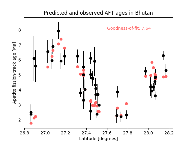
Example plot for Problem 1.
Calculating summations
There are several ways in which you can calculate a summation in Python, including using the sum() function.
However, it is often better to use a for loop for summing values, particularly if you are calculating values and don’t want to store their results separately from the summation.
Perhaps an example will make this clear:
In [7]: numbers = [1,2,3,4,5,6,7,8,9]
In [8]: squaredSum = 0 # Set sum equal to zero before starting for loop
In [9]: for i in range(len(numbers)):
...: squaredSum = squaredSum + numbers[i]**2.0
...:
In [10]: squaredSum
Out[10]: 285.0
In [11]: sum(numbers) # Sum of the list values
���������������Out[11]: 45
In [12]: sum(numbers)**2.0 # Square of the sum of the list values, not equal to squaredSum
���������������������������Out[12]: 2025.0
The point here is that in order to calculate the sum of each value squared in a Python list, you need to calculate the square of each value in the list separately, then add those together.
You could save the squared values in a separate list and use the sum() function, but in this case it may be more clear and logical to use a for loop.
You may want to do something similar for calculating your chi squared values.
Shorthand Python notation for adding to a variable
It is extremely common to need to add to an existing variable in computer programs. Because of this, there is a shorthand notation in Python for just this kind of operation.
In [13]: number = 34

In [14]: number = number + 5

In [15]: print(number)
39

In [16]: number += 5

In [17]: print(number)
44
As you can see, number += 5 is exactly the same as number = number + 5, just written a bit more compactly.
As you might imagine, there are similar shortcuts for subtracting (-=), multiplying (*=), and dividing (/=).
Problem 2
Example plot
Your code for this problem should produce plots similar to the two below.
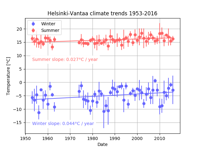
Example plot for Problem 2 with all years of climate data.
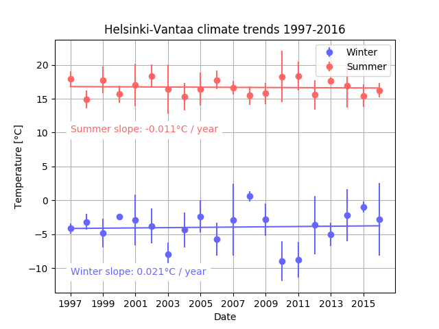
Example plot for Problem 2 with the last 20 years of climate data.
Reading in data with a datetime index
One of your first tasks in this problem is to read in a datafile that was generated from a Pandas DataFrame with a datetime index. There are several ways in which the data file can be read, but one of the easier options is to read it in with the necessary parameters to make sure the date information is properly treated as a datetime index. This will give you a DataFrame that is just like that you were using in Exercise 7 of the Geo-Python part of the course. To read in data where one column contains dates that should be used as the index, you can do the following:
data = pd.read_csv('some_file.csv', sep=',', index_col='dates', parse_dates=True)
Assuming that the name of the date column is dates, index_col specifies which column in the data file should be used as the index in the DataFrame, and parse_dates tells Pandas to treat the index column data as datetime values.
As mentioned, there are alternative options, but this is a clean way to read in data to Pandas with a datetime index.
Drop the nan values to avoid problems with the regression calculations
Once you have read in the climate data and filled in your DataFrame that contains the seasonal average temperatures and standard deviations in temperature, you’ll want to get rid of any nan (not a number) values for the seasonal temperatures.
The reason for this is that you will have problems calculating the A and B values if there are any nan values.
Consider the following example:
In [18]: testArray = np.linspace(0.0, 10.0, 11)
In [19]: print(testArray)
[ 0. 1. 2. 3. 4. 5. 6. 7. 8. 9. 10.]
In [20]: print(sum(testArray))
���������������������������������������������������������55.0
In [21]: testArray[4] = np.nan
In [22]: print(testArray)
[ 0. 1. 2. 3. nan 5. 6. 7. 8. 9. 10.]
In [23]: print(sum(testArray))
���������������������������������������������������������nan
In [24]: print(testArray[4] + testArray[5])
�������������������������������������������������������������nan
As you can see, if you sum or add values containing a nan your sum will be nan.
Unlike plotting data containing nan values, that is not good for sums.
Use .values to get array values for calculating A and B
When doing your regression line calculations you will want to be sure to be working with simple array data, rather than Pandas DataFrame data. What?!? Yeah, so it turns out that you can’t easily do math with Pandas DataFrame values, so you need to convert those values into a simpler structure. NumPy is the basis for the Pandas DataFrame, so it is quite easy to do this. Again, I’ll show an example.
In [25]: import pandas as pd
In [26]: testDF = pd.DataFrame(np.random.randn(4,2),columns=['Col1', 'Col2'])
In [27]: print(testDF)
Col1 Col2
0 -1.249509 0.554675
1 1.000981 0.233781
2 0.287120 0.877611
3 -0.808938 -0.265338
In [28]: testDF['Col1']
��������������������������������������������������������������������������������������������������������������Out[28]:
0 -1.249509
1 1.000981
2 0.287120
3 -0.808938
Name: Col1, dtype: float64
In [29]: testDF['Col1'].values
�����������������������������������������������������������������������������������������������������������������������������������������������������������������������������������������������������������Out[29]: array([-1.24950932, 1.00098074, 0.28711968, -0.80893791])
As you can perhaps see, testDF is a basic Pandas DataFrame with two columns Col1 and Col2 with random values.
Taking a single column from this DataFrame testDF['Col1'] returns a Pandas Series.
Alternatively, testDF['Col1'].values produces a NumPy array of that same data.
You will likely find that you’re not able to do your calculations of A and B for the regression lines unless you use the .values attribute.
Use the year for calculating the regression lines
You do not need the day and month when trying to calculate the regression lines. Instead, you only want the observation year. Assuming you have a datetime index for your data, you can get the years as follows:
In [30]: print(testDF)
Col1 Col2
0 -1.249509 0.554675
1 1.000981 0.233781
2 0.287120 0.877611
3 -0.808938 -0.265338
In [31]: index = pd.date_range('2013', '2016', freq='AS')
In [32]: testDF = testDF.set_index(index)
In [33]: print(testDF.index)
DatetimeIndex(['2013-01-01', '2014-01-01', '2015-01-01', '2016-01-01'], dtype='datetime64[ns]', freq='AS-JAN')
In [34]: print(testDF.index.year)
���������������������������������������������������������������������������������������������������������������Int64Index([2013, 2014, 2015, 2016], dtype='int64')
As you can see, if we add a datetime index to testDF, we can output the index range by typing print(testDF.index).
To get the equivalent data in years only, we print print(testDF.index.year).