Theory for Exercise 12

Problem 1

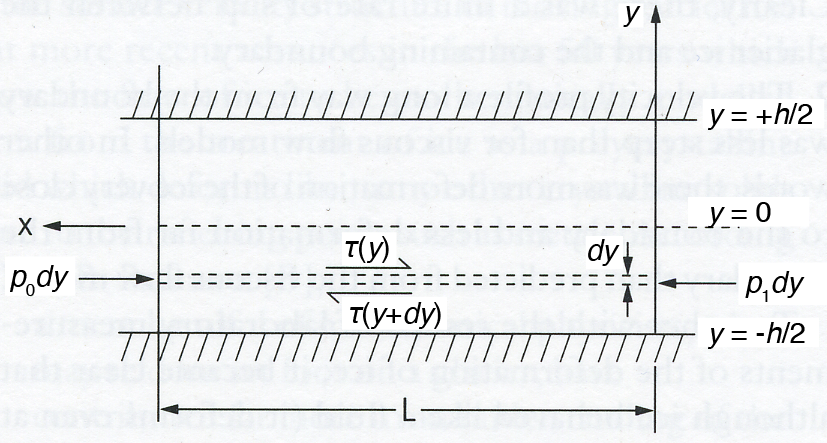
Figure 1. Schematic diagram of pressure-driven flow in a channel.

The viscosity of ice depends on both temperature and stress. For simplicity, we’ll consider the case where viscosity is only a function of shear stress. Consider a channel of width \(h\) centered about \(y = 0\), with lateral boundaries at \(y = \pm h/2\) (Figure 1). A pressure gradient \(\Delta p = p_{1} - p_{0}\) drives flow within the channel of length \(L\). The shear stress in the fluid depends on the applied pressure gradient and the distance from the channel boundaries

\[\frac{d \tau}{d y} = \frac{d p}{d x} = \frac{p_{1} - p_{0}}{L} \tag{1}\]

where \(\tau\) is the shear stress. We know that for Newtonian fluids

\[\tau = \eta \frac{d u}{d y} \tag{2}\]

where \(\eta\) is the dynamic viscosity of the fluid. Substituting the right side of Equation 2 into the left side of Equation 1 we find

\[\eta \frac{d^{2} u}{d y^{2}} = \frac{d p}{d x} \tag{3}\]

Integrating Equation 3 with respect to \(y\) twice we get

\[\begin{split}\begin{align} \int \frac{d^{2} u}{d y^{2}} &= \frac{1}{\eta} \int \frac{d p}{d x} \tag{Integrate once}\\ \frac{d u}{d y} &= \frac{1}{\eta} \frac{d p}{d x} y + c_{1} \tag{4} \\ \int \frac{d u}{d y} &= \frac{1}{\eta} \int \frac{d p}{d x} y + c_{1} \tag{Integrate again} \\ u(y) &= \frac{1}{2 \eta} \frac{d p}{d x} y^{2} + c_{1} y + c_{2} \tag{5} \end{align}\end{split}\]

Since we know \(d u / d y = 0\) at \(y = 0\), we find \(c_{1} = 0\), and because we assume zero slip at the boundaries of the channel (\(u = 0\) at \(y = \pm h / 2\)), \(c_{2} = (1 / 2 \eta)(d p / d x)(h / 2)^{2}\). Thus,

\[u(y) = \frac{1}{2 \eta} \frac{d p}{d x} \left[ y^{2} + \left( \frac{h}{2} \right)^{2} \right] \tag{6}\]

This is the velocity profile for a Newtonian fluid, but as you will recall, we learned that ice is a non-Newtonian (nonlinear viscous) fluid. As such, the behavior should be modeled using a power-law, where the strain rate is a related to the shear stress as follows

\[\frac{d u}{d y} = a \tau^{n} \tag{7}\]

where \(a\) is a function of the viscosity and temperature (we will ignore temperature for now), and \(n\) is the power-law exponent. If we solve Equation 7 in terms of \(\tau\), we can substitute the result into Equation 1 to get

\[a^{-1/n} \frac{d}{d y} \left( \frac{d u^{1/n}}{d y} \right) = -\frac{p_{1} - p_{0}}{L} \tag{8}\]

Assuming symmetry about the center line \(y = 0\) and integrating we see

\[\begin{split}\begin{align} \int \frac{d}{d y} \left( \frac{d u^{1/n}}{d y} \right) &= -a^{1/n} \int \frac{p_{1} - p_{0}}{L} \tag{Integrate} \\ \frac{d u^{1/n}}{d y} &= -a^{1/n} \frac{p_{1} - p_{0}}{L} y + c_{1} \tag{Raise both sides to the power n} \\ \frac{d u}{d y} &= -a \left( \frac{p_{1} - p_{0}}{L} \right)^{n} y^{n} + c^{n}_{1} \tag{Apply BC $\frac{d u}{d y} = 0 \bigg\rvert_{y=0}$} \\ \frac{d u}{d y} &= -a \left( \frac{p_{1} - p_{0}}{L} \right)^{n} y^{n} \tag{9} \end{align}\end{split}\]

Note

In the derivations, boundary condition has been abbreviated as BC to save space.

Now integrate Equation 9 and assume \(u = 0\) at \(y = \pm h / 2\).

\[\begin{split}\begin{align} \int \frac{d u}{d y} &= -a \left( \frac{p_{1} - p_{0}}{L} \right)^{n} \int y^{n} \\ u(y) &= -\frac{a}{n + 1} \left( \frac{p_{1} - p_{0}}{L} \right)^{n} y^{n + 1} + c_{2} \tag{Apply BC $u = 0$ at $y = \pm \frac{h}{2}$} \\ u(y) &= \frac{a}{n + 1} \left( \frac{p_{1} - p_{0}}{L} \right)^{n} \left[ \left( \frac{h}{2} \right)^{n + 1} - y^{n + 1} \right] \tag{10} \end{align}\end{split}\]

The mean velocity in the fluid is

\[\begin{split}\begin{align} \bar{u} &= \frac{2}{h} \int_{0}^{h/2} u dy \\ &= \frac{a}{n + 2} \left( \frac{p_{1} - p_{0}}{L} \right)^{n} \left( \frac{h}{2} \right)^{n + 1} \tag{11} \end{align}\end{split}\]

We can calculate a non-dimensional velocity now by dividing the velocity at any point in the channel by the mean velocity

\[\frac{u}{\bar{u}} = \left( \frac{n + 2}{n + 1} \right) \left[ 1 - \left( \frac{2 y}{h} \right)^{n + 1} \right] \tag{12}\]

Problem 2

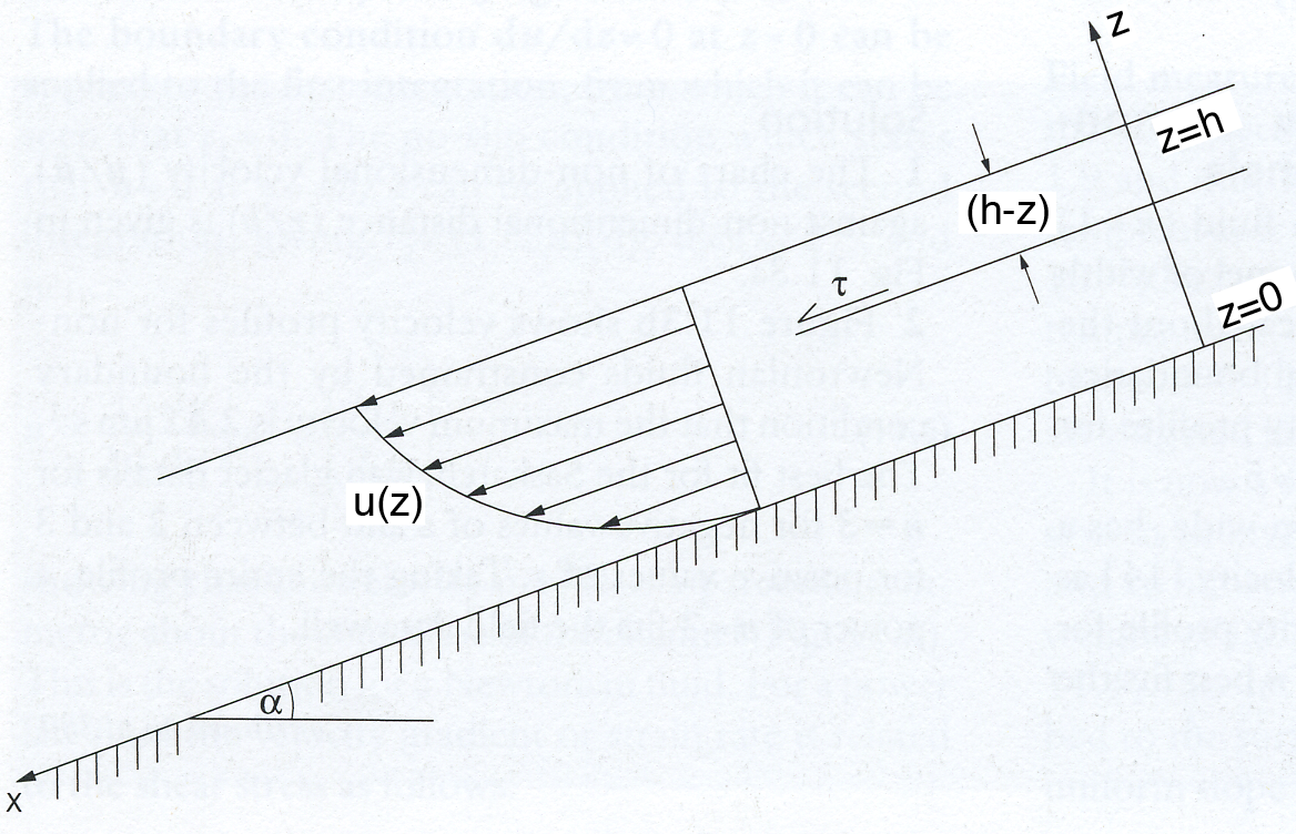
Figure 2. Schematic diagram of a viscous fluid flowing down an inclined plane.

The velocity of a fluid flowing down an inclined plane can be modelled using some basic physical relationships. First, recall that the basal shear stress for a fluid flowing down an inclined plane is due to the down slope component of the weight of the overlying fluid

\[\tau = \rho g h \sin{\alpha} \tag{13}\]

where \(\rho\) is the fluid density, \(g\) is the acceleration due to gravity, \(h\) is the thickness of the fluid perpendicular to the inclined plane and \(\alpha\) is the angle of the plane with respect to horizontal. At any distance \(z\) above the bed

\[\begin{split}\begin{align} \tau &= \rho g (h - z) \sin{\alpha} \\ &= \gamma_{x} (h - z) \tag{14} \end{align}\end{split}\]

where \(\gamma_{x} = \rho g \sin{\alpha}\) is the downslope component of the gravitational force. Combining Equation 2 from Part 1 of the theory with Equation 14 we find the constitutive equation for a Newtonian fluid is

\[\frac{d u}{d z} = \frac{\gamma_{x} (h - z)}{\eta} \tag{15}\]

Integrating Equation 15 yields

\[\begin{split}\begin{align} \int \frac{d u}{d z} &= \int \frac{\gamma_{x} (h - z)}{\eta} \\ u(z) &= \frac{\gamma_{x}}{\eta} \left( z h - \frac{z^{2}}{2} \right) + c_{1} \tag{16} \end{align}\end{split}\]

where \(c_{1} = 0\) from the boundary condition \(u = 0\) at \(z = 0\). Equation 16 can be rewritten as

\[u(z) = \frac{1}{2} \left( \frac{\gamma_{x}}{\eta} \right) \left[ h^{2} - (h - z)^{2} \right] \tag{17}\]

For a non-Newtonian fluid, Equation 14 can be modified to account for the case where the strain rate varies as a power of the shear stress (Equation 7 from Part 1 of the theory)

\[\frac{d u}{d z} = a \left[ \gamma_{x} (h - z) \right]^{n} \tag{18}\]

To determine the velocity profile, we need to integrate Equation 18. If we use the boundary condition that the basal sliding velocity is equal to ub rather than zero, we get

\[\begin{split}\begin{align} \int \frac{d u}{d z} &= a \int \left[ \gamma_{x} (h - z) \right]^{n} \\ u(z) &= u_{\mathrm{b}} + \frac{a}{n + 1} \gamma_{x}^{n} \left[ h^{n + 1} - (h - z)^{n + 1} \right] \tag{19} \end{align}\end{split}\]